

Usual column filters in Google Sheets paintings smartly for some datasets, however they’re hidden within menus, require edit get admission to to make use of, and clear out a unmarried desk at a time. Slicers sit down on most sensible of your sheet as floating, clickable controls that anybody can use (without reference to get admission to). Additionally they replace each hooked up pivot desk and chart at the sheet the instant you are making a variety. Right here’s find out how to upload slicer to Google Sheets, customise the way it seems to be, and use some complex choices for the use of it.
How you can Upload Slicer to Google Sheets
Slicers paintings absolute best when your knowledge is in a structured desk the place you may have column headers within the first row, no merged cells, and no clean rows breaking apart the knowledge. In case your spreadsheet already has a pivot desk or chart constructed from an outlined vary, the slicer will pick out up that vary robotically. In the event you’re operating with a flat knowledge desk, you’ll be able to click on any place within the desk earlier than including the slicer so Google Sheets can establish the proper vary by itself.
Step 1. Click on on any cellular throughout the knowledge vary you need to clear out. If you wish to connect the slicer to a chart or pivot desk you’ve already constructed, click on at the chart or pivot desk as a substitute. Make sure you prepare your knowledge with column headers within the first row, without a clean rows or merged cells.
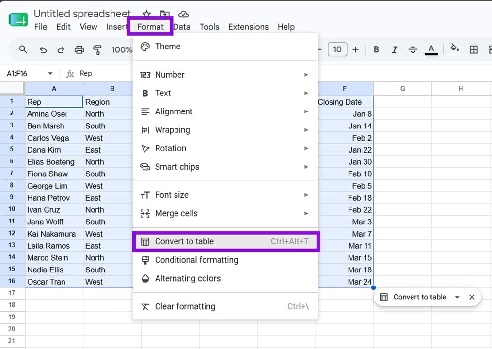
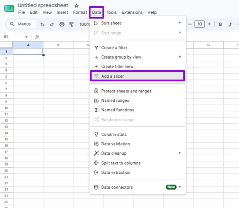
Step 2. Cross to the highest menu, click on “Knowledge,” and select “Upload a slicer.”
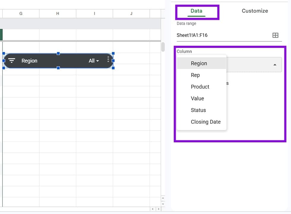
Step 3. Within the sidebar, below the Knowledge tab, you’ll see a knowledge vary box. Google Sheets in most cases fills this in in line with your variety. If it’s clean or mistaken, click on the grid icon subsequent to the sphere and choose the proper vary, or kind it in manually (as an example, A1:F216).
Step 4. Nonetheless within the Knowledge tab, open the Column dropdown and select which column the slicer must keep an eye on.
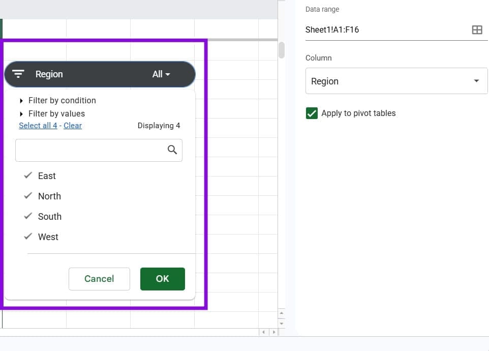
As for find out how to use slicer in Google Sheets, you wish to have to click on on its dropdown arrow. You’ll see a listing of all distinctive values within the column you selected, and you’ll be able to take a look at or uncheck knowledge.
How you can Customise the Slicer’s Look
As soon as a slicer is for your sheet, you’ll be able to regulate the way it seems to be.
To open the customization choices, double-click at the slicer and move to the “Customise” tab at the sidebar. From there, you’ll be able to exchange the slicer’s name – it defaults to the column title, however you’ll be able to rename it to one thing extra readable – the name font, measurement, and formatting, the background colour of the slicer field, and the textual content colour.
To resize the slicer, click on on it to make a choice it and drag the handles on its edges.
While you’ve styled a slicer the best way you need it, you’ll be able to use it as a template for extra slicers by means of clicking the three-dot menu and deciding on “Replica slicer,” then pasting it onto the sheet. The reproduction inherits the similar look settings, so that you solely wish to exchange the column it filters.
How you can Upload A couple of Slicers for Multi-Column Filtering
One slicer controls one column. As an example, if you wish to clear out your knowledge by means of Area and by means of Product on the similar time, you wish to have two separate slicers.
So as to add a 2d slicer for a unique column, repeat the similar procedure as with the primary and select a 2d column for it, or create a replica of the prevailing slicer.
There’s no arduous prohibit on what number of slicers you’ll be able to upload, however maximum tables will cap out at 3 or 4. Past that, believe whether or not a clear out view or a pivot desk with file filters would serve the use case higher.
Thank you to your comments!