5 Excel errors inexperienced persons make that break their spreadsheets (and what to do as an alternative)

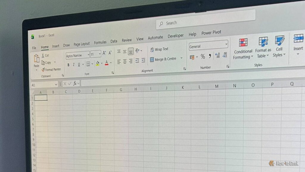
There is a large distinction between a spreadsheet that appears excellent and one who in reality works. Many novice spreadsheet behavior are secretly ticking time bombs in your information. Listed here are the core errors messing up your information, and the straightforward settings that repair them.

Merging cells ruins your information sorting and filtering

Use Middle Throughout Variety to stay your rows intact

If an information level spans a whole row, your intuition could be to make a choice the cells and click on “Merge & Middle” to create a blank, spanning label. Whilst it appears tidy at the floor, merging cells breaks Excel’s skill to regard your information as a constant, predictable grid. Excel can now not correctly kind or filter out levels that comprise merged cells, frequently triggering an error.

A greater manner is a integrated format trick that spans your textual content visually with out changing the underlying grid construction:

1. Make a selection the cells around the row the place you need the access to look targeted.
2. Press Ctrl+1 to open the Structure Cells conversation, then open the Alignment tab.
3. Underneath the Horizontal drop-down menu, select Middle Throughout Variety, then click on OK.

Your textual content will glance just like a merged mobile, however each column beneath stays utterly impartial, that means your filters and sorting possible choices will paintings as anticipated.

Formatting information manually breaks your formulation whilst you upload new rows

Flip your information blocks into respectable Excel tables

When inexperienced persons construct an inventory in Excel, they generally simply get started typing into clean cells, manually follow background colours, and impressive the highest row. It could seem like a desk to you, however to Excel, it is a disconnected pile of random information.

This turns into an issue whilst you sort formulation on the backside of a column, like summing up your totals. When you upload 5 new rows of information day after today, your system may not mechanically replace to incorporate them as a result of it is hard-coded to a static vary—you need to manually drag the system down or redefine the variability each unmarried time.

To avoid this handbook maintenance:

1. Be certain that your information has a unmarried header row and preferably accommodates no utterly clean rows or columns.
2. Click on any place throughout the information block.
3. Press Ctrl+T (or click on Insert > Desk) to transform it into an Excel desk.
4. Verify that the right kind vary is chosen and your information has headers, then click on OK.

Excel now treats the knowledge as a structured desk that expands mechanically.

Excel tables immediately structure your information with alternating row colours, however the true magic is within the capability. As a result of tables are absolutely dynamic, including a brand new row on the backside mechanically expands the desk to house it. Formulation and charts attached to the desk replace mechanically because the desk grows, and PivotTables seize the brand new information after refresh.

OS

Home windows, macOS, iPhone, iPad, Android

Loose trial

1 month

Microsoft 365 contains get admission to to Place of work apps like Phrase, Excel, and PowerPoint on as much as 5 units, 1 TB of OneDrive garage, and extra.

Hiding rows and columns manually makes your information simple to lose

Crew your information to stay your workspace blank and toggleable

When a spreadsheet will get cluttered with previous information or helper columns, right-clicking the ones rows or columns and settling on Disguise seems like a very easy win.

However hidden rows are extremely simple to omit about, resulting in confusion when totals do not fit. Even worse, copying information with hidden rows can produce surprising effects relying on how the choice is made.

As a substitute of hiding information blindly:

1. Make a selection the rows or columns you need to tuck away.
2. Open the Knowledge tab at the ribbon.
3. Click on Crew.

Excel then provides a visible bracket to the margin in your spreadsheet with a easy plus (+) or minus (-) toggle button, which you’ll click on to cave in or enlarge blocks with a unmarried click on.

This helps to keep your structural good judgment completely visual whilst shielding your spreadsheet from pointless muddle.

Blending textual content and numbers in the similar column breaks your calculations

Follow strict information varieties to stay formatting uniform

In well-structured Excel datasets, each and every row is a document (a unmarried access, like a transaction) and each and every column is a box (a particular characteristic—like a date, worth, or amount—consisting of a unmarried information sort).

The difficulty begins whilst you sort unit symbols, forex indicators, or textual content modifiers immediately right into a mobile along a host—like coming into “100 lbs” or “$50” manually. Once you sort a letter or an emblem right into a numeric box, Excel treats all the access as textual content moderately than a numeric price. Consequently, Excel would possibly exclude the ones cells from numeric calculations.

A greater manner is to let Excel grasp the uncooked quantity within the box whilst the usage of the Quantity Structure engine to deal with the visible presentation:

1. Kind most effective natural numbers into your column (corresponding to 100 as an alternative of $100 or 100 lb).
2. Make a selection the column or information vary.
3. Open the House tab at the ribbon.
4. Increase the Quantity staff drop-down (which defaults to “Basic”).
5. Make a selection the related quantity structure, or open Extra Quantity Codecs to outline a customized unit label (like #,##0″ lbs”).

By means of keeping apart the visible look from the true information sort, your information keep readable for people whilst nonetheless utterly calculable for Excel.

Arduous-coding numbers within formulation creates a repairs nightmare

Use devoted enter cells to stay your good judgment dynamic

When writing formulation that contain mounted values—like a 5% tax—it is tempting to easily sort the quantity immediately into the system. A calculation like:

=[@Cost]*1.05

appears blank, works completely, and will get the activity achieved.

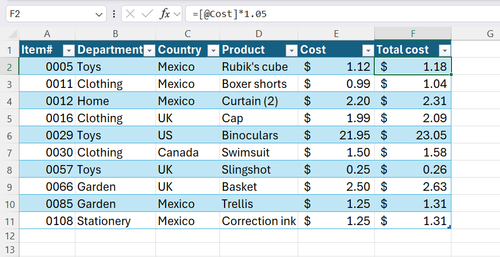
On the other hand, the issue presentations up later when that price adjustments. If the tax charge will increase to six%, each hard-coded reproduction of that quantity turns into a repairs downside. In higher workbooks, lacking even one example can quietly distort your totals.

A greater manner is to split your assumptions out of your calculations by way of making a devoted enter sheet in your variables:

1. Click on the + icon on the backside of your window so as to add a brand new sheet.
2. Double-click the brand new sheet and rename it to Assumptions.
3. Within the new sheet, position the assumptions in column B, and their related labels in column A (as an example, “Tax” in A1 and “0.05” in B1).
4. Make a selection all assumptions and labels, then click on Formulation > Create from Variety.
5. Within the conversation field, take a look at Left Column, then click on OK.

You’ll now reference the assumptions immediately in formulation like this:

=[@Cost]*Tax

Now, when the tax charge adjustments, updating only one mobile impacts all the workbook.

Say good-bye to damaged sheets

Swapping out handbook behavior for local Excel equipment like tables, grouping, mobile inputs, and Middle Throughout Variety guarantees your workbooks stay solid {and professional}. Now that you know the way to keep away from those commonplace formatting hazards, you’ll hopefully construct spreadsheets that scale. To place those blank behavior into apply these days, attempting a couple of novice Excel initiatives is an effective way to sharpen your talents.